Description of the Shock tool :

Authors: K. Dalmasse, A. Kouloumvakos, A.P. Rouillard, M. Alexandre, M. Indurain

Scientists/Engineers: A.P. Rouillard (IRAP, CDPP-STORMS, Ionospheric Research Center, IRAP-Thalès), K. Dalmasse (IRAP, CDPP-STORMS, IRCIT)

System engineer/web developer: M. Indurain (InforMarty), M. Alexandre ((IRAP, CDPP-STORMS, IRCIT)

External support from the FORSPEF team: A. Papaioannou (IAASARS/NOA), A., Anastasiadis (IAASARS/NOA) and the NOA team.

I. Introduction

Summary: The shock tool is a fast 3D coronal shock wave propagation module developed to provide quick modeling of shock wave properties in the corona and establish how these shocks connect magnetically to specific points of interest in the inner heliosphere. These shock waves accelerate energetic particles to high energy and this approach is therefore a first step towards forecasting Solar Energetic Particles (SEPs), the latter feature will be fully implemented in a future update of the tool. At this stage, the Shock Tool forecasts the 3-D expansion speed of a CME shock wave erupting from a specific Active Region (AR). This does not comprise the cases of CMEs ejected from inter-ARs or outside the activity belt. The Active Regions are the NOAA ARs as detected on the visible disk. The model assumes a spherical expansion of the shock and an apex speed provided by forecasts and/or empirical models of CME speeds. Shock modeling is only one part of the story, in order to predict the impact of a coronal shock on a specific region of the inner heliosphere (such as the Earth), we must determine how the particle accelerator connects magnetically to that region. Magnetic connectivity is retrieved from the Infor’marty magnetic connectivity tool and already available in the Heliospheric Expert Center (H.ESC).

Acronyms :

• AM : Alfvén Mach number
• AR : Active Region
• CME : coronal mass ejection
• FL : field lines
• FM : Fast magnetosonic Mach number
• GLEs : Ground Level Enhancements
• MHD : Magneto-Hydrodynamics
• SEPs : Solar Energetic Particles

SWx goals of the tool: to provide nowcasts and forecasts of propagating shocks on magnetic field lines connected to spacecraft and planets in the inner heliosphere. The tool provides forecast of shock waves propagating towards the interplanetary medium. Shocks can produce harmful SEPs and knowledge that a shock wave is likely to form in relevant regions of the solar atmosphere constitutes a first step towards anticipating and monitoring the sources of these SEPs and Ground Level Enhancements (GLEs) that can not only affect spacecraft but also aicraft.

Future upgrades of the tool: The Shock Tool provides forecasts and nowcasts of the time-evolution of key shock parameters such as the Alfvén and Fast-Mode Mach number of the shock that quantify the strength of a shock wave and its ability to accelerate particles to high energy. In a future upgrade of the tool, we will exploit known relations between the intensity of SEPs and Mach numbers (Kouloumvakos et al. 2019) to provide nowcasts and forecasts of the flux of SEPs in different energy bands. The Shock Tool will also provide the velocity vector at all points on the surface of the shock, this has been used in a different version of the application as initial conditions to 3-D MHD models including HELIOCAST (Réville et al. 2023) and EUHFORIA (Pomoell and Poedts, 2018). A second upgrade of the tool will allow coupling of the Shock Tool with these 3-D MHD interplanetary models. In the future, the tool will also provide ecliptic plots of the heliospheric propagation of the modeled shock wave, together with a basic SEP index (yes/no) based on the shock wave Mach number. Other potential upgrades will be related to improving the presentation of the tool, to highlight in color the NOAA data in nowcasting mode when it uses observational data and exhibits some activity. We will also integrate updates to the Magnetic Connectivity Tool including a visualisation of the shock wave propagating through the magnetic field lines. An API is also under construction in order to select plots from past events.

Validation/comparison with observational data: a validation of the tools forecasting capabilities is in progress and will be the topic of an upcoming publication. This will involve an evaluation of the forecasts of shock waves arrival times with in situ measurements at L1 and other position in the heliosphere of IP shocks. The next upgrade of the tool will include forecasts of SEP events and a validation of the performances of the tool will also be carried out by comparing the SEP forecasts with in situ measurements of energetic particles.

Mach number and importance of shock criticality: Coronal shocks undergo different regimes that are related to the value of their Mach number which provides a quantification of the strength of a shock wave and its ability to accelerate particles to high energies thereby producing SEPs. The processes by which particles are accelerated at shock waves are not well understood, statistical work analysing a large set of SEP events in terms of their connection to shock waves, shows that the higher the Mach number the higher the SEP event (Kouloumvakos et al. 2019), this is supported by advanced models of particle acceleration (Afanasiev et al. 2018). There is a critical Mach number (Mann 1995) above which simple resistivity cannot provide the total shock dissipation and a shock begins altering significantly the energy of the particles in its vicinity. The microphysical structure of collisionless shocks is very different when the shock is sub- or super-critical (e.g., Marcowith et al. 2016). In the super-critical case a significant amount of upstream ions are reflected on the shock front, gaining an amount of energy that enables them to be injected into the acceleration process. Sub-critical shocks do not reflect ions, significantly diminishing the ion and electron acceleration efficiency. Mc is a function of the various shock parameters including the shock geometr defined by the angle that the shock normal makes relative to the magnetic field direction. It has been argued that it is at most 2.7 and usually much closer to unity (e.g., Mann 1995). The critical Mach number varies from around 1.53 for parallel shocks to about 2.76 for perpendicular shocks (Kouloumvakos et al. 2019). In the Shock Tool, we consider a universal threshold in that a shock is termed super-critical when MFM>3 and is then considered a potential efficient particle accelerator capable of producing SEPs.

II. Use of product and interpretation of plots

Web-interface to forecasts/nowcasts of coronal shocks

The web-interface of the Shock Tool is in place to provide to the users a visualisation of forecasts/nowcasts of shock wave properties and extract critical information about their propagation. The interface shown in Figure 1 provides the modeled shock parameters and quick information about their impact at different points in the heliosphere based on the results of the nowcasting or forecasting mode. The tool provides the evolution of the shock parameters at magnetically well-connected field lines with the different spacecraft.

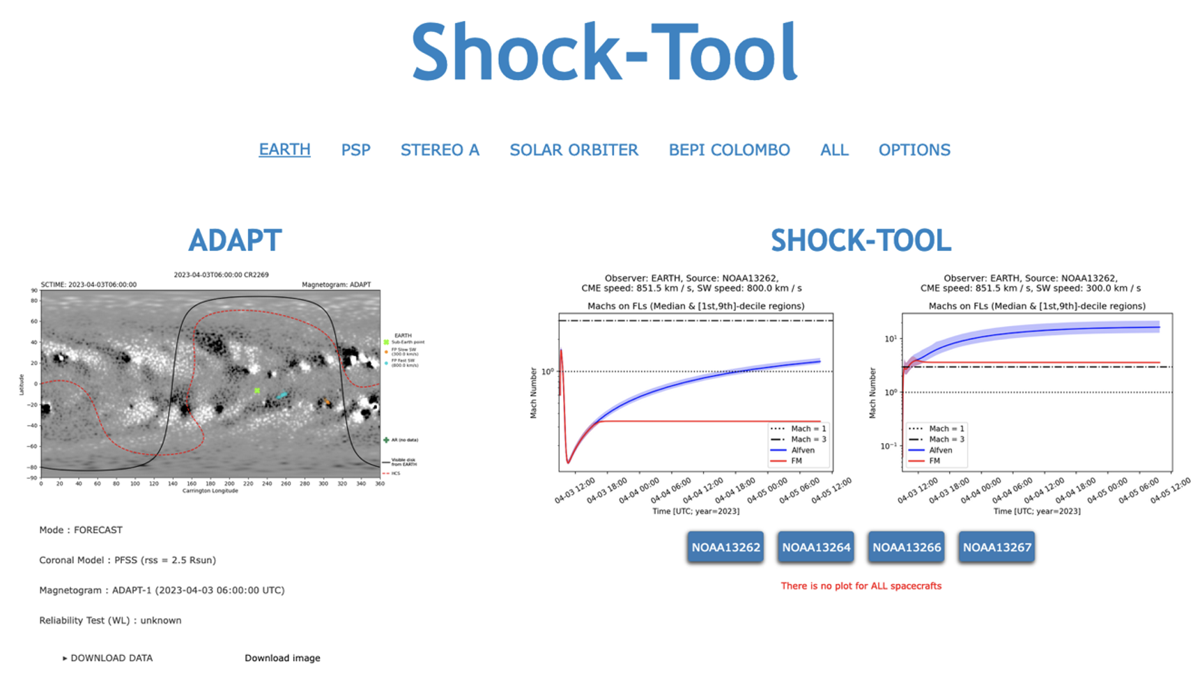
Visualisation of forecasted shock wave properties is provided for all ARs for which the IAASARS/NOA delivers a CME speed forecast (forecasting mode), and for all on-disk ARs reported by Solar Monitor (nowcasting mode). The tool provides shock properties forecasts along magnetic field lines connected to all the observers/spacecraft for which the Infor’marty Magnetic Connectivity tool delivers a magnetic connectivity forecast. The interface displays the temporal profiles of the modeled shock Mach numbers and compares them to the critical Mach values that are favorable for the production of SEP events.

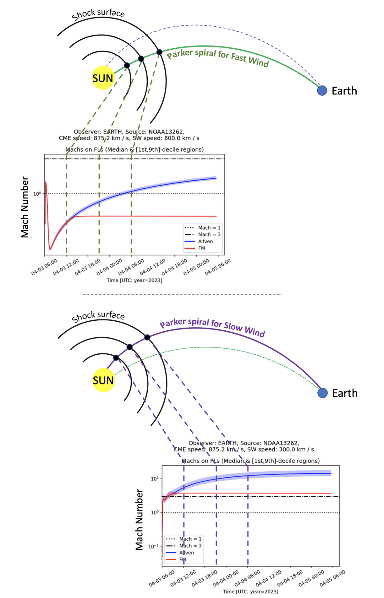
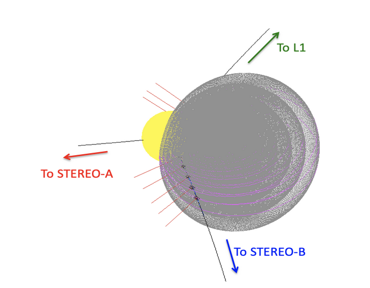
The timelines shown in the interface represent the conditions of CME shock ejected along a magnetic field connected to the spacecraft selected in the interface and originating from the AR also selected in the interface. We provide two sets of predictions based on whether a spacecraft connects to the shock via interplanetary magnetic field lines defined by a slow (300 km/s) or fast (800 km/s) solar wind. This is illustrated in Figure 2. Indeed, since the interplanetary magnetic field lines connected to the shock are defined by the solar wind speed, the region of the shock a spacecraft will be magnetically connected to will be very different in the two types of solar wind. Since we do not know the speed of the solar wind in advance, we suppose these two extrema (300 and 800 km/s).
- The blue lines in each plot present forecasts of the time varying Shock Alfvén Mach number along magnetic field lines connected to the selected spacecraft and originating in the selected AR.
- The red line presents forecasts of the time varying Fast Magnetosonic (FM) Mach number along magnetic field lines connected to the selected spacecraft and originating in the selected AR.
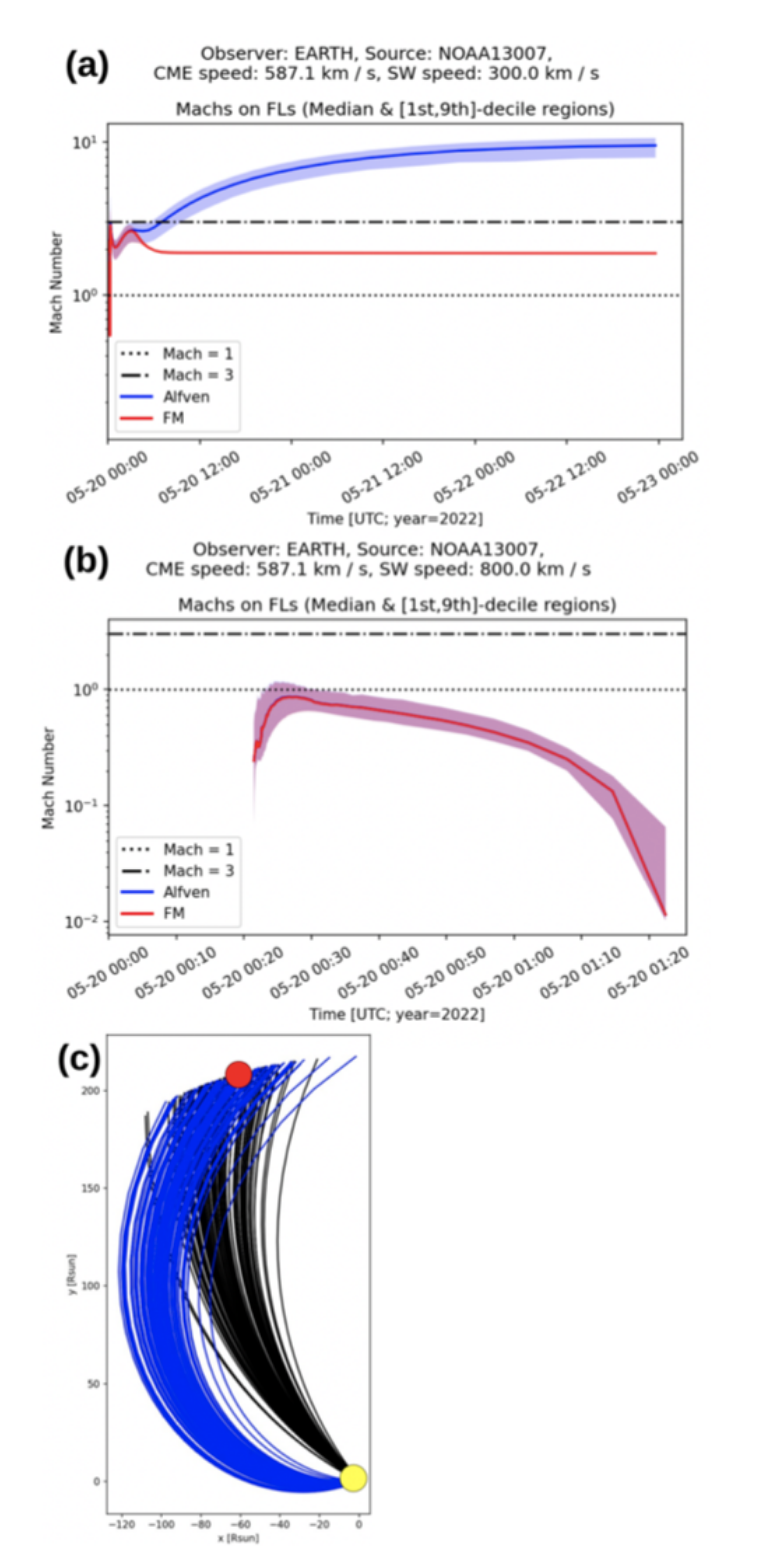
Typically, a scatter-free 1GeV proton will take 10 minutes to reach Earth when considering fast solar wind, and a scatter-free 1GeV proton will take 12 minutes when considering slow solar wind. Start time of the product: the plots starts at real time in UTC, and the plots are updated every 6 h, from the magnetic connectivity tool, as described below. When the lines cross the threshold of M=1 (dotted line), one can consider that a shock is likely to have formed in the solar corona, and when the lines cross the threshold of M=3 (dashed-dot line), the shock is likely to have become super-critical and start accelerating particles to high energy. The timeline is a proxy of an spatial representation: if a M>1 is passed very close to the hypothetical ejection/shock time, it may imply that that the shock is produced closer to the Sun’s corona. The uncertainties of the forecasted Mach numbers are on the 1 and 9 deciles (10 and 90 percentiles) are obtained statistically by an ensemble of Parker spirals, this is illustrated in Figure 3. This ensemble of field lines is provided by the Infor’Marty magnetic connectivity tool and defined by criteria given in the associated tutorial. It provides an estimate of the uncertainty of magnetic connectivity by considering a bundle of Parker spiral distributed around the nominal Parker spiral trajectory.

The product does not provide an API.

III. Models used, input data and limitations:

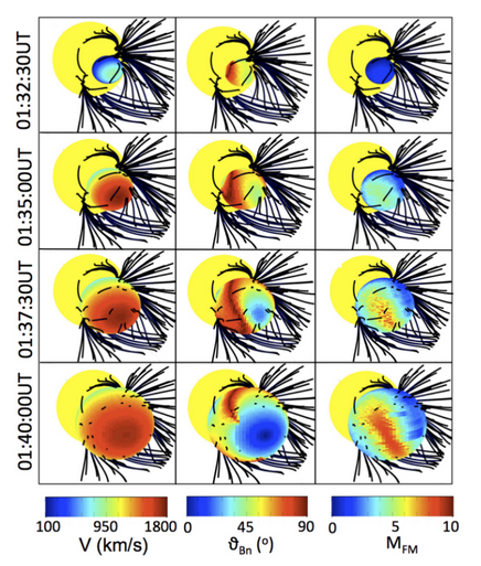
The challenge: The Shock Tool tackles the challenging task of modeling the high variability of a shock wave as it progresses through the highly structured corona and inner heliosphere. This variability is illustrated in Figure 4 taken from Rouillard et al. (2016). Because of this spatial and temporal variability of the shock, the conditions for the acceleration of SEPs can be very different at different locations of the shock surface. A particular spacecraft connecting magnetically to the flank of the shock will not measure the same intensity of SEPs as the same spacecraft connecting near the supercritical nose of the shock. This has been shown statistically by Kouloumvakos et al. (2019) and addressed with a physics-based modelling of SEP acceleration along the shock surface shown in Figure 1 of Afanasiev et al. (2018).

Physics-based modelling of SEP acceleration is very time consuming (hours to days of computational time) and not yet feasible for SEP forecasts necessary within seconds of our knowledge of an on-going solar event. Therefore the approach of the Shock Tool has been to adopt a compromise: to address the variability of the shock by considering both its time-evolving complex magnetoplasma structure as well as the way spacecraft and planets connect magnetically to that shock since energetic particles are guided by these fields lines.

The tool is an adaptation of the coronal shock model of Rouillard et al. (2016) that has been further developed and exploited to study the origin of strong particle events (Kouloumvakos et al. 2019) and electromagnetic radiation from radio waves to gamma rays (Kouloumvakos et al. 2020, 2021). In its scientific version, the 3-D expansion speed of shock waves is obtained by first fitting geometrical shapes (spheres, ellipsoids) representing the shock to direct images of the shock wave imaged by extreme ultraviolet telescopes (such as SDO/AIA) and white-light coronagraphs (such as SoHO LASCO C2/C3). The other shock properties are then derived by exploiting background coronal and solar wind models. In the present operational tool we do not fit the 3-D shock shape to real-time imagery but assume a spherical and self-similar expansion. The speed of the apex of the spherical shock is either provided by external forecasting services (forecasting mode) or computed using an empirical model (nowcasting mode). The tool was made highly modular in order to run both in forecasting and nowcasting modes. Currently the forecasting and nowcasting modes are running in tandem, in such a way that only the results associated with the latest prediction are made available.

In the forecasting mode, the shock parameter calculations are performed for the ARs that have a high probability of eruption (ARs flaring probabilities). The probabilities of flaring and producing CMEs are provided by the The FORecasting Solar Energetic Particles and Flares (FORSPEF) tool put in place by IAASARS/NOA (https://www.astro.noa.gr/en/) http://tromos.space.noa.gr/forspef/main/ and described in Papaioannou et al. (2015). The Shock Tool uses the forecasts of CME occurrence and speed issued by the For the implementation of the forecasting system of solar flare, a novel method was developed based upon the effective connected magnetic field strength (Beff) metric and it utilizes analysis of a large number of active region (AR) magnetograms (more detail given in M. K. Georgoulis & D. M. Rust, Astrophys. J. 2007, 661, L109). For a given AR, under the condition of a specific calculated Beff value, the system implemented under FORSPEF, derives conditional-probabilities for solar flares for broad intensity range (C1.0 - X10), the respective CME-likelihood for each flare class, as well as, a projected near-Sun CME velocity relying on the given Beff value independently inferred.

In the nowcasting mode, however, the shock calculations are performed for all on-disk ARs reported by the Solar Monitor webservice (https://www.solarmonitor.org/) and triggered by the real-time detection of flare events reported by NOAA/SWPC from the GOES X-Ray flux data (https://www.swpc.noaa.gov/products/goes-x-ray-flux). The empirical relation of Salas-Matamoros et al. (2015) is then used to estimate a hypothetical CME/shock speed from the GOES X-Ray flux, considering the relation between eruptive flares and CMEs only, with a caveat of not considering confined flares, and the clarification that the integrated GOES X-ray full integrated flux does not provide information about the nature of the flare or its position in the solar disk. The nature of the CMEs is upper solar atmosphere material ejected due to instabilities triggered by strong releases or energy. These are typically triggered by eruptive filaments lying in a Polarity Inversion Line (PIL), inside or outside ARs. This empirical relation is used to roughly estimate a hypothetical CME speed that could be related to the nowcasted flare. No LASCO C2/C3 data or other coronagraph (e.g. STEREO) is used for nowcasting.

Shock modeling is only one part of the story, in order to predict the impact of a coronal shock on a specific region of the inner heliosphere (such as the Earth), we must determine how the particle accelerator connects magnetically to that region. Magnetic connectivity is retrieved from the Infor’marty magnetic connectivity tool developed in support of Solar Orbiter operations (http://stormsconnectsolo.irap.omp.eu/) and already available in the Heliospheric Expert Center (H.ESC). This tool already runs in forecast or nowcast modes.

The forecasting and nowcasting procedure for the shock 3D expansion previously described is combined with such forecasts/nowcasts of magnetic connectivity to refine the computed shock properties (speed, Mach, geometry) along field lines of interest.

IV. Technical description of the Shock Tool

We have implemented a Python package to perform the shock wave expansion modeling. The package enables the forecasting of a spherical shock wave expansion.

The forecasting mode relies on predictions of CME occurrence and speed delivered by the IAASARS/NOA (https://www.astro.noa.gr/en/) at a 3-hour cadence through their Advanced Solar Particle Events Casting System (ASPECS) http://phobos-srv.space.noa.gr/api/fl_cme_fore_json, used as input for the forecasting mode. This facility operated by IAASARS/NOA through the FORSPEF project (Papaioannou et al. 2015) provides continuous forecasts of solar eruptive events, including solar flares and CME occurrence probabilities and estimated forecasted speed (as well as the likelihood of a SEP event and the complete SEP profile). The Shock Tool uses these forecasts of CME speeds issued by NOA for each considered AR on the solar disk to set the speed of the apex of the spherically-expanding shock emerging from the considered AR. The forecasting mode does not allow to estimate shock perturbations triggered by multiple CMEs from the same AR, and therefore does not consider multiple shock interactions.

The nowcasting mode is triggered and replaces the forecasting mode for a specific AR when a solar X-ray flare is reported by NOAA/SWPC’s latest flare event report typically updated every 1-minute. The Shock Tool exploits these reports to compute and update an hypothetical CME speed based on the real-time X-Ray flux measurements by the GOES satellites, since direct CME observation by LASCO C2/C3 is not used in this tool The speed of the hypothetical CME is then estimated from the GOES X-Ray flux based on the CME speed-flare relations of Salas-Matamoros et al. (2015) considering the relation between eruptive flares and CMEs only. This has a caveat of not considering confined flares, and/or all the other conditions that are not adequate to trigger instabilities and subsequently filaments eruptions and subsequently CMEs.

The nowcasting mode does not allow to estimate shock perturbations triggered by multiple CMEs from the same AR, and therefore does not consider multiple shock interactions. This approach supposes that the hypothetical CME speed and the shock speed are the same. It also considers that the CME speeds used in Salas-Matamoros et al. (2015) are true deprojected speeds. This is not true since the authors used LASCO C2/C3-derived CME speeds that are inherently projected speeds. This will be replaced in a future upgrade by new relations derived between X-ray measurements and deprojected shock speeds derived from the shock 3-D fitting (Jarry et al. 2023). In a future upgrade of the tool where we will also provide SEP forecasts we will compare our SEP forecasts with those issued by the FORSPEF project which also provides nowcasting of SEP events based on actual solar flare and CME near real-time alerts.

The forecasting and nowcasting modes are running in tandem, in such a way that only the results associated with the latest prediction are made available. For instance if a flare is detected in an AR by the GOES satellites, then as soon as NOAA releases a maximum flare intensity, the Shock Tool ceases to run in forecasting mode in that AR and instead uses the maximum flare intensity provided by NOA to redefine the probability of a CME and its subsequent estimated speed of the CME from related AR). Examples of Shock Waves simulated by the tool are given in Figure 5.

Magnetic Connectivity of the Shock: In order to connect the correct part of the shock wave with a spacecraft or planet that might be influenced by an SEP event triggered by that same shock, the Shock Tool fetches the magnetic field line coordinates connected to each spacecraft/planet computed by Infor’marty Magnetic Connectivity Tool and already available through ESA SWE Service Network Portal. The magnetic field lines are delivered by the Magnetic Connectivity Tool at a 6-hour cadence. These magnetic reconstructions are based on a combination of extrapolations of ADAPT magnetograms with flux transport, together with a simple Parker spiral model for the interplanetary medium (Rouillard et al. 2020). Low speed solar wind produce a more curved Parker spiral, while the fast solar wind is traced by a bit more straight Parker spirals (as already illustrated in Figures 2 and 3). A future version of the tool will include magnetic connectivity models derived from more complex and realistic solutions, e.g., Wind-Predict (Réville et al. 2020) or PSI-MAS (MHD, Lionello et al. 2009), or substituting the simple interplanetary Parker spiral with the results of EUHFORIA simulations (Pomoell and Poedts 2018) coupled to MULTI-VP (Pinto and Rouillard 2016).

Derivation of shock properties: The modeled 3D shock wave is currently limited to a spherical wave in self-similar expansion at a constant speed, more complex shock geometries will be considered during future upgrades (e.g., new geometries, time-varying shock speed). In order to compute the shock’s Mach number along the connected magnetic field lines we must assume a form of the background solar wind through which the shock is propagating. Currently the properties of the background solar wind are obtained from a set of pre-defined analytical coronal/solar wind plasma models. In a future upgrade the tool will exploit more self-consistent physics-based background Solar Wind models (e.g., MULTI-VP).

Acknowledgements: The Shock Tool was originally developed during the H2020 EUHFORIA 2.0 project, it is now integrated in the ESA SWE Service Network Portal.

References:

• Afanasiev A., Vainio R., Rouillard A.P., Battarbee M., Aran A., Zucca P., 2018, A&A, 614, A4. doi:10.1051/0004-6361/201731343
• Georgoulis M K and Rust D M 2007 The Astrophysical Journal Letters 661 L109
• Jarry, M., Rouillard, A.P., Plotnikov, I., Kouloumvakos, A., 2023, Astronomy & Astrophysics, Volume 672, id.A127, 11 pp.
• Kouloumvakos A., Rouillard A.P., Wu Y., Vainio R., Vourlidas A., Plotnikov I., Afanasiev A., et al., 2019, ApJ, 876, 80. doi:10.3847/1538-4357/ab15d7
• Kouloumvakos A., Rouillard A.P., Share G.H., Plotnikov I., Murphy R., Papaioannou A., Wu Y., 2020, ApJ, 893, 76. doi:10.3847/1538-4357/ab8227
• Kouloumvakos A., Rouillard A., Warmuth A., Magdalenic J., Jebaraj I.C., Mann G., Vainio R., et al., 2021, ApJ, 913, 99. doi:10.3847/1538-4357/abf435
• Lionello, R., et al., The Astrophysical Journal, Volume 690, Issue 1, pp. 902-912 (2009).
• Mann G., 1995, LNP, 183. doi:10.1007/3-540-59109-5_50
• Marcowith, A., Bret, A., Bykov, A., et al. 2016, RPPh, 79, 046901, doi: 10.1088/0034-4885/79/4/046901
• Papaioannou, A., Anastasiadis, A., Sandberg, I., Georgoulis, M.-K., Tsiropoula G., Tziotziou, K., Jiggens, P., Hilgers, A., 2015 J. Phys.: Conf. Ser. 632 012075, doi:10.1088/1742-6596/632/1/012075
• Pinto, R.F. Rouillard, A.P., The Astrophysical Journal, 838, Issue 2, 89,
• Pomoell J., Poedts S., 2018, JSWSC, 8, A35. doi:10.1051/swsc/2018020
• Réville, V., Velli, M., et al., The Astrophysical Journal Supplement Series, Volume 246, Issue 2, id.24, 11 pp. (2020)
• Réville, V., Poirier, N., Kouloumvakos, N., Rouillard, A.P., Journal of Space Weather and Space Climate, Accepted for publication in the Journal of Space Weather and Space Climate, 2023
• Rouillard A.P., Plotnikov I., Pinto R.F., Tirole M., Lavarra M., Zucca P., Vainio R., et al., 2016, ApJ, 833, 45. doi:10.3847/1538-4357/833/1/45
• A. P. Rouillard, R. F. Pinto, A. Vourlidas, et al 2020, A&A ,642, A2 https://doi.org/10.1051/0004-6361/201935305
• Salas-Matamoros C., Klein K.-L., 2015, SoPh, 290, 1337. doi:10.1007/s11207-015-0677-0